VLOOKUP returns the wrong row in Google Sheets (TRUE approximate match)

You look up sku 200 and VLOOKUP hands back Lamp, not Chair. The formula ran. It matched the wrong row.

Recreate it on a blank sheet

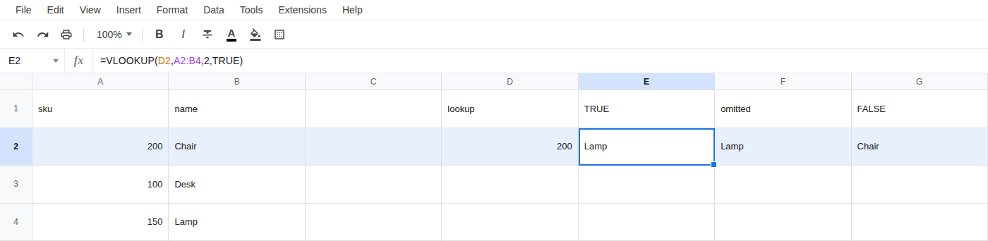
1. Open a blank spreadsheet. In A1 type sku, B1 name. Leave column C empty. D1 lookup, E1 TRUE, F1 omitted, G1 FALSE.
2. Type the table in this order — 200 first, then 100, then 150. A2 200, B2 Chair. A3 100, B3 Desk. A4 150, B4 Lamp. In D2 type 200.
3. In E2 enter =VLOOKUP(D2,A2:B4,2,TRUE). The cell shows Lamp.

4. In F2 enter =VLOOKUP(D2,A2:B4,2) with no fourth argument. That cell is also Lamp. Omitting the fourth argument is the same as TRUE.

What is actually wrong

• The fourth argument is the match mode. TRUE means approximate match. Leaving it off is the same as TRUE.
• Approximate match walks the first column as if it were sorted ascending. This list is not: 200, then 100, then 150.
• Sku 200 is sitting in A2 next to Chair. Approximate match still returns Lamp from the last row.
• FALSE is exact match. It finds 200 and returns Chair.

Fix

For sku lookups, always pass FALSE. Leave E2 and F2 as the broken formulas so the wrong row stays on the sheet.

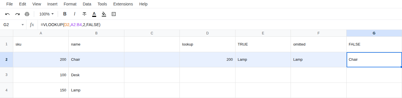
In G2 enter =VLOOKUP(D2,A2:B4,2,FALSE). The cell shows Chair.

Sku lookups are exact. FALSE is the argument that does that. Do not sort the table to make TRUE look right — that is not the fix.