You can see the lookup value with your eyes and VLOOKUP still returns #N/A. That is usually not a missing row. It is a key that does not actually match.
Recreate it on a blank sheet
- Open a blank spreadsheet. In A1 type
sku, B1name, D1lookup, E1result. - In A2 type
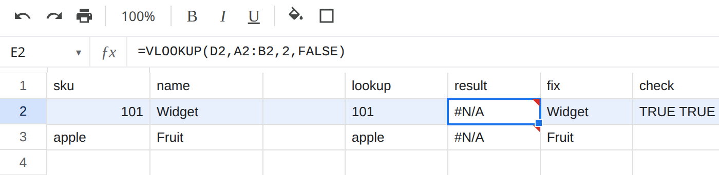
101as a number. B2Widget. In D2 type an apostrophe then101so Sheets stores it as text. In E2 enter=VLOOKUP(D2,A2:B2,2,FALSE). The cell shows#N/A.
- In A3 type
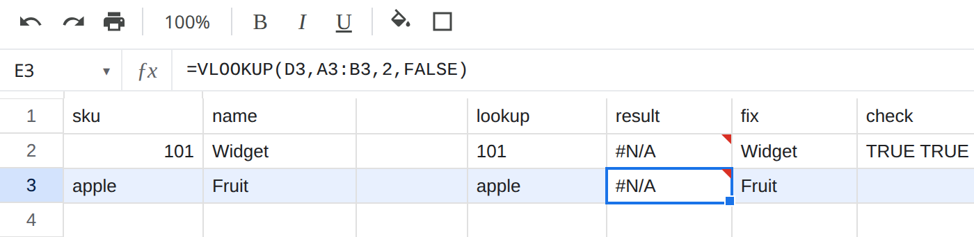
applethen a space. B3Fruit. D3applewith no space. In E3 enter the sameVLOOKUPagainstA3:B3. That cell is also#N/A.
What is actually wrong
- Numbers and text are not the same key.
101the number is not'101the text.VLOOKUPwithFALSEdoes not coerce them. - A trailing space in the table is a different string.
appleis notapple. TRIMon the lookup value only does not fix a space that lives in the table column.
Check: =LEN(A3) is 6. =LEN(D3) is 5.
Fix
- Number column:
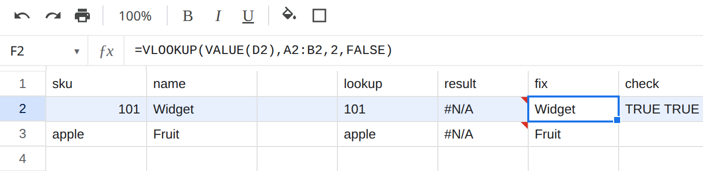
=VLOOKUP(VALUE(D2),A2:B2,2,FALSE)returns Widget. If the table were text and the lookup a number, wrap the table key instead.
- Space in the table: trim the table side, for example
=VLOOKUP(D3,{TRIM(A3),B3},2,FALSE)returns Fruit. For real data,TRIMthe sku column, not only the lookup cell.
If it looks equal and VLOOKUP disagrees, check type and LEN before you rewrite the formula.